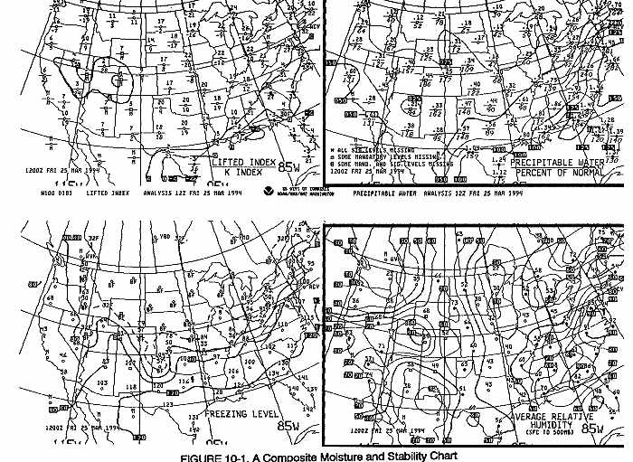
COMPOSITE MOISTURE STABILITY CHART
The composite moisture stability chart (Figure 10-1), is an analysis chart using observed upper air data. The chart is composed of four panels including stability, freezing level, precipitable water and, average relative humidity. This computer-generated chart is available twice daily with valid times of 12Z and 00Z. The availability of upper air data (on all the panels) for analysis is indicated by the shape of the station model. Use the legend on the precipitable water panel of Figure 10-4 for the explanation. On this chart, the mandatory levels used are the surface, the 1000 mb/hPa, the 850 mb/hPa, the 700 mb/hPa, and the 500 mb/hPa. Significant levels are the levels where significant changes in temperature and/or moisture occur when compared to below or above that level.
STABILITY PANEL
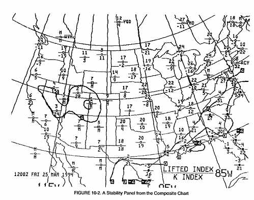
The stability panel, the upper left panel of the chart, outlines areas of stable and unstable air. Figure 10-2 shows the two stability indices that are computed for each upper air station. The top value is the lifted index and is plotted above a short line, below the line is the K index. An "M" indicates the value is missing.
Lifted Index (LI)
The lifted index is computed as if a parcel of air near the surface were lifted to 500 millibars/hectoPascals (18,000 feet MSL). As the air is "lifted" it cools, at 3 degrees Celsius per 1,000 feet, due to expansion. The temperature the parcel would have at 500 millibars is then subtracted from the actual (environmental) 500 millibar/hectoPascal temperature. This difference is the lifted index which is positive, negative or zero and indicates the stability of the parcel of air.
A positive index means that a parcel of air, if lifted, would be colder than the surrounding air at 500 millibars/hectoPascal. The air is, therefore, stable and would resist vertical motion. Large positive values (+8) would indicate very stable air.
A negative index means that the low-level air, if lifted to 500 millibars/hectoPascals, would be warmer than the surrounding air. The air is unstable and suggests the possibility of convection. Large negative values (-4 or less) would indicate very unstable air.
A zero index means that the parcel of air, if lifted to 500 millibars/hectoPascals, would have the same temperature as the actual air at 500 millibars/hectoPascals. This air is said to be neutrally stable (neither stable or unstable).
When using this chart, remember that the lifted index assumes the air near the surface will be lifted to 500 millibars/hectoPascals. Whether or not the air near the surface will be lifted to 500 millibars/hectoPascals depends on what is happening below. It is possible to have a negative LI with no thunderstorm development because either the air below 500 mb/hPa is not being lifted high enough or there is not enough moisture in the air. For use, the lifted index is more indicative of the severity of the thunderstorms, if they occur, rather than the probability of general thunderstorm occurrence (Table 10-1). Also note that the LI can change dramatically just by daytime heating and nighttime cooling. Daytime heating tends to make the LI value less positive (more unstable) and nighttime cooling tends to make the LI more positive (more stable).
K Index
The K index is primarily for the meteorologist. It examines the temperature and moisture profile of the environment. The K index is not really a stability index because the parcel of air is not lifted and compared to the environment. The K index is computed using three terms:
K = (850 mb/hPa temp - 500 mb/hPa temp)
+ (850 mb/hPa dew point)
- (700 mb/hPa temp/dew point
spread)
The first term (850 mb/hPa temp - 500 mb/hPa temp) compares the temperature at about 5,000 feet MSL to the temperature at about 18,000 feet MSL. The larger a temperature difference, the more unstable the air and the higher the K value.
The second term (850 mb/hPa dew point) is a measure of low-level moisture. Note that since the dew point is added to the value, high moisture content at 850 mb/hPa increases the K value.
The third term (700 mb/hPa temp/dew point spread) is a measure of saturation at 700 mb/hPa. The greater the spread, the drier the air; and since the term is subtracted, it lowers the K value. The greater the degree of saturation at 700 millibars/hectoPascals, the larger the K value.
During the thunderstorm season, a large K index indicates conditions favorable for air mass thunderstorms (Table 10-1). However, K index values and meanings can decrease significantly for thunderstorm development associated with a synoptic scale low pressure system (non air-mass thunderstorms).
In winter, because of cold temperatures and low moisture values, the temperature terms completely dominate the K value computation. Because of the lack of moisture, even fairly large values do not mean conditions are favorable for thunderstorms. Be aware that the K values can change significantly over a short time period due to temperature and moisture advection.
It is essential to note that an unstable Lifted Index does NOT automatically mean thunderstorms. Look at the synoptic situation and if thunderstorms are expected to develop in the unstable air, Table 10-1 may be used in accordance with this section.
* Use caution when applying these values in the western mountainous terrain due to elevation.
Stability Analysis
The analysis is based on the lifted index only. Station circles are blackened for LI values of zero or less. Solid lines are drawn for values of +4 and less at intervals of 4 (+4, 0, -4, -8, etc).
Using the Panels
When clouds and precipitation are forecast or are occurring, the stability index is used to determine the type of clouds and precipitation. That is, stratiform clouds and continuous precipitation occur with stable air, while convective clouds and showery precipitation occur with unstable air.
Stability is also very important when considering the type, extent, and intensity of aviation weather hazards. For example, a quick estimate of areas of probable convective turbulence can be made by associating the areas with unstable air. An area of extensive icing would be associated with stratiform clouds and steady precipitation which are characterized by stable air.
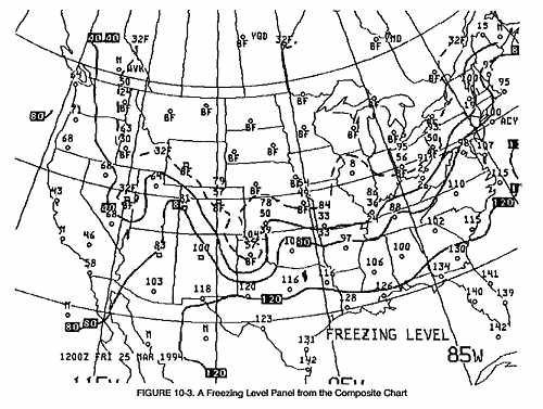
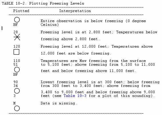
FREEZING LEVEL PANEL
The freezing level panel, the lower left panel of the chart, is an analysis
of the observed freezing level data from upper air observations (Figure
10-3).
|
NOTE: The asterisk and the box, instead of a circle, indicate some of the data is missing.
All heights are above Mean Sea Level (MSL).
Analysis
Solid lines are contours of the lowest freezing level and are drawn for 4,000 foot intervals and labeled in hundreds of feet MSL. When a station reports more than one crossing of the zero degree Celsius isotherm, the lowest crossing is used in the analysis. This is in contrast to the low-level significant weather prog on which the depicted forecast freezing level aloft is the highest freezing level. A dashed line represents the 32 degree Fahrenheit isotherm at the surface and will outline an area of stations reporting "BF" (below freezing).
Using the Panel
The contour analysis shows an overall view of the lowest observed freezing level. Always plan for possible icing in clouds or precipitation especially between the temperatures of zero and -10 degrees Celsius.
Plotted multiple crossings of the zero degree Celsius isotherm always show an inversion with warm air above subfreezing temperatures (Table 10-3). This situation can produce very hazardous icing when precipitation is occurring. Airmet ZULU (Section 4) shows more specifically the areas of expected icing. The low-level significant weather prog shows anticipated changes in the freezing level.
TABLE 10-3. Vertical Temperature Profile of Freezing Levels.
This is an example of three crossings of the 0 degree C isotherm.
PRECIPITABLE WATER PANEL
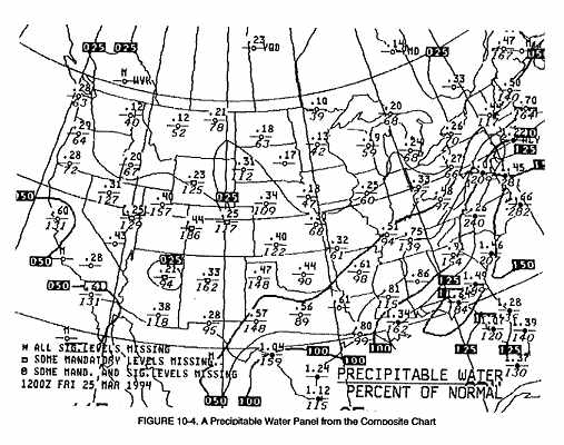
The precipitable water panel, the upper right panel of the chart, is an analysis of the water vapor content from the surface to the 500 mb/hPa level (Figure 10-4). The amount of water vapor observed is shown as precipitation water, which is the amount of liquid precipitation that would result if all the water vapor were condensed.
Plotted Data
At each station, precipitable water values to the nearest hundredth of an inch are plotted above a short line and the percent of normal value for the month below the line. The percent of normal value is the amount of precipitable water actually present compared to what is normally expected. In Figure 10-4, Amarillo, Texas has a plot of ".47/148." This indicates that 47 hundredths of an inch of precipitable water is present which is 148 percent of normal (above normal) for any day during this month. The ".44/90" at Oklahoma City indicates that 445 hundredths of an inch of precipitable water is present which is only 90 percent of normal (below normal) for any day during this month. An "M" plotted above the line indicates missing data as shown at the station in Canada north of Washington. At Huron, SD the percent of normal value is not plotted. This indicates insufficient climatological data to compute this value.
Analysis
Stations with blackened in circles indicate precipitable water values of 1.00 inch or more. Isopleths (lines of equal values) of precipitable water are drawn and labeled for every 0.25 inches with heavier isopleths drawn at 0.50 inch intervals.
Using the Chart
This panel is used to determine water vapor content in the air between surface and 500 mb/hPa (18,000 feet MSL). It is especially useful to meteorologists concerned with flash flood events. By looking at the wind field upstream from a station, one can get an indication of changes that will occur in the moisture content; that is, determine if the air is drying out or increasing in moisture with time.
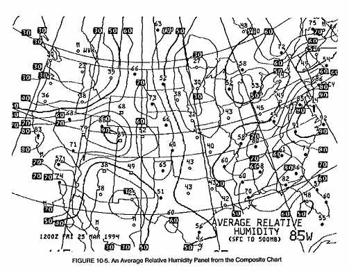
AVERAGE RELATIVE HUMIDITY PANEL
The average relative humidity panel, the lower right panel of the chart, is an analysis of the average relative humidity from the surface to 500 mb/hPa. The values are plotted as a percentage for each reporting station (Figure 10-5). An "M" indicates the value is missing.
Analysis
Station circles are blackened for humidities of 50 percent and higher. Isopleths of relative humidity, called isohumes, are drawn and labeled every 10 percent with heavier isohumes drawn for values of 10, 50 and 90 percent.
Using the Panel
This panel is used to determine the average air saturation from the surface to 500 mb/hPa. Average relative humidities of 50 percent and greater are quite frequently associated with areas of clouds and possibly precipitation. Clouds and possible precipitation can be assumed, due to the high average relative humidity through approximately 18,000 feet. It is likely that a layer or layers will have 100 percent relative humidity with clouds and possibly precipitation. It is important to remember that high values of relative humidity do not necessarily mean high values of water vapor content (precipitable water). For example (Figure 10-4), Las Vegas, NV has less water vapor content than New Orleans, LA (.43 and 1.34 respectively). However, in Figure 10-5, the average relative humidities are nearly the same for both stations. If rain were falling at both stations, the result would likely be lighter precipitation totals for Las Vegas.
USING THE COMPOSITE MOISTURE STABILITY CHART
This chart is used to determine the characteristics of a particular
weather system in terms of stability, moisture, and possible aviation hazards.
Even though this chart is several hours old when received, the weather
system will tend to move these characteristics with it. Caution should
be exercised as modification of these characteristics could occur through
development, dissipation, or the movement of the system.